In this post and the next we will survey an assortment of intrinsic properties groups can enjoy that bear vestiges of non-positive curvature. We will focus here on hyperbolicity, which stands out as a compelling notion of negative curvature for a group. In next post we will discuss incorporating zero–curvature — the field of reasonable properties then becomes wider.
Suppose that a group  is CAT(0) or CAT(-1) — that is, it acts properly cocompactly by isometries on a CAT(0) or CAT(-1) space
  . The motivation behind the definitions of most intrinsic properties of non-positive curvature comes from identifying geometric features of non-positive curvature in — such as CAT(-1) spaces having uniformly thin triangles and the metrics in CAT(0) spaces being convex — and recognising the implications they have for .
The following lemma (whose proof we will omit) helps us translate between groups and spaces on which they act. It’s first conclusion — finite generation — means can be given a word metric, as is required to make sense of the second conclusion.
The Svarc–Milnor Lemma (e.g. Bridson and Haefliger, page 140). If a group acts on a geodesic space (or, indeed, a length space) properly and cocompactly by isometries, then is finitely generated and for any choice of base point  , the map
  is a quasi-isometry
  .
.
Fix a finite generating set  for . Let
  be a quasi-inverse for
  — that is, a quasi-isometry for which there is some
  with the property that
 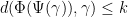 and
and 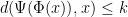 for all
  and
and  . We have focused on features of CAT(0) and CAT(-1) spaces that concern their geodesics. When we carry a geodesic
 ![{[0,r] \rightarrow X}](https://s0.wp.com/latex.php?latex=%7B%5B0%2Cr%5D+%5Crightarrow+X%7D&bg=ffffff&fg=000000&s=0&c=20201002) to by composing it with
to by composing it with  , it is no longer a geodesic — it becomes a quasi–geodesic, by which mean a
  –quasi–isometric embedding
 ![{\rho: [0,r] \rightarrow \Gamma}](https://s0.wp.com/latex.php?latex=%7B%5Crho%3A+%5B0%2Cr%5D+%5Crightarrow+%5CGamma%7D&bg=ffffff&fg=000000&s=0&c=20201002) . Here, the constants
. Here, the constants  and
and  are uniform: they depend only on the constants associated to the quasi-isometry .
These  will usually not be continuous. It will prove convenient to tame them: they map to , which we identify with the vertices of the Cayley graph
  ; we can replace by a nearby edge–path
  — that is, a path that traverses successive edges in . This will be at the expense of replacing and by some larger uniform constants. (In more detail, construct by using shortest edge-paths to successively join
  to
to  for each pair of integers
  and
and  in
in ![{[0,r]}](https://s0.wp.com/latex.php?latex=%7B%5B0%2Cr%5D%7D&bg=ffffff&fg=000000&s=0&c=20201002) .)
.)
Definition. A geodesic space is  –hyperbolic when all its geodesic triangles are –thin.
As we’ve explained, CAT(-1) spaces are –hyperbolic for some  .
.
Lemma (Bridson and Haefliger, page 401–405). In a -hyperbolic geodesic space, a quasi-geodesic between two points is always uniformly close to any geodesic that connects those two points.
It is hard to explain why this important lemma is true without getting embroiled in the mass of inequalities involved in a formal proof. At the risk of being so vague as to be unintelligible, here’s a quick account of a three-stage proof. The first stage is to show that in a -hyperbolic geodesic space, if  is a path of length
  , then every point on a geodesic
  connecting the end–points of lies with in a distance
  of the path. One can see that this is true in
  : any path between the end points of a geodesic that detours around a
  -ball around a point on that geodesic must have length
  . Spanning a region between and with a collection of -thin triangles, we find that the metric in this region behaves similarly to that in in this respect. The second stage is that quasi-geodesics are uniformly close to continuous quasi-geodesics, and so we can consider continuous quasi-geodesics instead of arbitrary ones. This is similar to the taming we discussed above. The tamed quasi-geodesic then falls under the scope of stage one, and the third stage is to argue that the additional constraints on it that make it a quasi-geodesic lead to the stronger conclusion that it stays uniformly close to any geodesic between its end points.
Corollary. Geodesic triangles in the Cayley graphs of CAT(-1) groups are uniformly thin.
This motivated:
Definition (Hyperbolic group). A group with finitely generating set is -hyperbolic when its Cayley graph  is -hyperbolic. A finitely generated group is (Gromov-) hyperbolic when it is -hyperbolic for some finite generating set and some .
Gromov set out many of the properties of these groups in his paper Hyperbolic groups, Essays in group theory, 75–263, MSRI Publ., 8, Springer, 1987. Early and influential exegeses were provided by Ghys and de la Harpe (Sur les groupes hyperboliques d’après Mikhael Gromov, Progr. Math., 83, Birkhauser, 1990), and by Alonso, T. Brady, Cooper, Ferlini, Lustig, Mihalik, Shapiro and Short (also ed.). An English translation by Grosso of part of Ghys and de la Harpe’s account is available.
The notion is robust in that if is -hyperbolic for some finite generating set and  is another finite generating set, then will be
  -hyperbolic for some . Indeed, if
  is a finitely generated group that is quasi-isometric to , then will also be hyperbolic. [The lemma above about quasi-geodesics being close to geodesics in a –hyperbolic space is the key point in the proof.]
Examples. For examples of hyperbolic groups, we refer the reader to the list of CAT(-1) groups in our previous post — we’ve shown in our discussions above that all CAT(-1) groups are hyperbolic. As for non–CAT(-1) examples, an outstanding question in the field is —
Open question. Are all hyperbolic groups CAT(-1)? Indeed, are they CAT(0)?!
Alternate definitions of hyperbolic groups
A reason the notion of a hyperbolic group is compelling is that there are a number of markedly different, yet equivalent, ways to characterise them. In addition to the thin triangles condition, these include:
- They are the finitely generated groups whose asymptotic cones are all
 -trees.
- They are the finitely presented groups with linear Dehn functions.
- They are the finitely presented groups with subquadratic Dehn functions.
Number (1) is described by Gromov as the most natural characterisation — somewhat intimidatingly as the details of the definition of an asymptotic cone are technical. An -tree is a geodesic space whose geodesics triangles are all tripods — that is, are  -thin. An asymptotic cone of a metric space
  is a limit as
  of the sequence of spaces
  in which the metric is scaled. More crudely, it is a limiting impression of
  viewed from increasingly distant vantage points. [The definition calls on a non-principal ultrafilter to ensure convergence.] The essential point is that the –thin triangles of a –hyperbolic group become -thin in its cones.
Dehn functions, the focus of (2) and (3), are simultaneously geometric and algorithmic invariants of groups. They are geometric in that they are analogues of the following classical notion of an isoperimetric function  for a space: is the minimal (or infimal) number such that every loop of length at most
  can be spanned by a disc of area at most . Dehn functions are algorithmic in that they relate to the Word Problem for the group: whether there exists an algorithm which, on input a word on the generators, will declare whether or not that word represents the identity.
Most likely, we will return to Dehn functions in a later post, but here’s a somewhat vague definition which will suffice for now. Assume that every loop in the Cayley graph can be subdivided into loops of length at most some constant — this is equivalent to assuming the group is finitely presentable. The Dehn function  is the function
  defined so that is the minimal number such that every loop of length at most in admits a subdivision into no more than subloops of length at most .
Up to the following standard equivalence, does not depend on the choice of finite generating set or on . For functions  we write
  when
when  and
and  , and we write when there exists
  such that for all ,

When we say a group has linear Dehn function we mean  .
.
We will not prove (2) but here’s a sketch of a result that gets close: we’ll establish an upper bound of  .
.
Lemma. In a –hyperbolic group, there exists such that geodesics triangles whose the side–lengths are at most can be subdivided into  subloops of length at most
  . The idea of the proof is that each vertex on a side of the triangle can be joined by a path of length at most to a vertex on another side so as to subdivide the triangle into subloops, the largest of which is, potentially, a hexagonal loop meeting all three sides of the triangle:

Fills an arbitrary loop of length in by dividing it into three arcs of length  and then joining their end points by geodesics; then divide each of the three arcs into two of length
  , and then four of length
  and so on; connect up endpoints of the arcs with geodesics as shown below. Subdivide the centre geodesic triangle into
  subloops as per the lemma, then subdivide the three triangles in the next layer using
 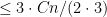 subloops, then the next layer with
 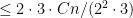 subloops, and so on. Stop when the geodesic triangles have sides of length at most some constant — that is after
  layers. The total number of subloops used is .

Much more work is required to improve this to  . There is an account here (Proposition 4.11) by Hamish Short of an elegant proof due to Noel Brady that hyperbolic groups have Dehn presentations. Getting follows readily.
The fact that groups with subquadratic Dehn function are hyperbolic implies that there are no Dehn functions between linear and quadratic. By contrast  is
is  the Dehn function of a group for a dense set of
  in the interval
  .
.
So from the point-of-view of Dehn functions, hyperbolic groups are a distinguished class, separated from all other finitely presentable groups by the interval  — the “Gromov gap”.
Good properties of hyperbolic groups
…there are many. Here are some highlights:
- They have no
 subgroups — this will be explained in a future post.
- They have Dehn presentations — see e.g. Bridson and Haefliger, p.448.
- Their geodesic words (words that are minimal length for the group elements they represent) form a regular language — this stems from a more geometric property of having finitely many cone types.
- They satisfy strong finiteness properties — they are finitely presented (as we essentially proved above), but even better those that are torsion free have a finite
 — specifically, the quotient of the Rips Complex by .
- It is easy to solve the word and conjugacy problems for a hyperbolic group — see e.g. Bridson and Haefliger.
- The isomorphism problem is decidable for hyperbolic groups (but is far from easy!) — for the torsion-free case see Sela, The isomorphism problem for hyperbolic groups. I., Ann. of Math. (2), 141(2):217–283, 1995; Sela also had a proof in the general case but did not publish it; Dahmani and Groves generalised Sela’s work, and then last year Dahmani and Guirardel gave a proof for the class of all hyperbolic groups.
Update, 18th February 2011: added to the references in point 6.


Are there any current candidates for groups that are hyperbolic but not CAT(-1)?
I’m no expert, but it’s easy to write down examples of hyperbolic groups, and in general there doesn’t seem to be a reason why these examples should be CAT(-1).
For instance, if an automorphism of a free group
  doesn’t fix any conjugacy classes then the free-by-cyclic group
  is hyperbolic, but in general I don’t know a reason why it should be CAT(-1).
Similarly, any group whose relations satisfy the small-cancellation condition is hyperbolic, but again I don’t think a reason is known for such a group to be CAT(-1). (See Lyndon & Schupp for the definition of
  .)
.)
The last example can be generalised to Gromov’s random groups, which are (with overwhelming probability) hyperbolic whenever they are infinite. Yet again, I don’t think any reason is known for such a group to be CAT(-1). (Though in some small ranges they are known to be CAT(0), by work of Ollivier and Wise.)
Your link to the proof that hyperbolic groups have linear Dehn functions is broken, so I thought I’d say a few words about it.
I like this proof because it’s a nice example of the sort of local-to-global argument that shows up everywhere when you talk about hyperbolic groups. Basically, one version (I’m not sure if this is Noel’s version or not) goes like this:
Let $K$ be a sufficiently large number. Let $w:[0,l(w)]\to C_\Gamma(A)$ be a loop.
Say that there are $0\le x,y\le l(w)$ such that $|x-y|\le K/2$ and $d(w(x),w(y))< |x-y|$. Then we can shorten $w$ by replacing that segment of $w$ with a geodesic. If every sufficiently large loop can be shortened this way, that means that the group has a linear Dehn function — this reduction process corresponds to a decomposition into loops of length $K$ (this property that every loop can be shortened is what it means for the group to have a Dehn presentation).
So, say that $w$ is a loop which cannot be shortened like this. Then $w$ is a $K/2$-local geodesic (that is, a curve such that if $|x-y|\le K/2$, then $d(w(x),w(y)) = |x-y|$). It turns out that $K/2$-local geodesics are in fact quasi-geodesics when $K$ is sufficiently large (the local-to-global argument I mentioned). This takes some work, but the main tool is the fact that quasi-geodesics are close to geodesics. So now, $w$ is a curve which is within a neighborhood of the geodesic between its endpoints, but that geodesic is just the constant curve, so $w$ has bounded length and the group has a linear Dehn function.
Thanks, Robert! The link is now fixed.
The approach you describe is the one taken by Hamish/Noel, except the business of local-geodesics being quasi-geodesics and quasi-geodesics being close to geodesics is bypassed… or perhaps, more accurately, is nicely distilled to the bare essence that is need to prove the result.