The following is largely based on the paper The Tits Alternative for CAT(0) Cubical Complexes by Sageev and Wise.
1.1. The Tits alternative
A group  satisfies the Tits alternative if for all subgroups
  , either
  is virtually solvable or it contains a non-abelian free group. One way to think of this is that a group satisfying the Tits alternative has either “small” subgroups (subgroups and quotients of solvable groups are solvable), or “large” subgroups (extensions by groups containing a free group contain a free group). The term originates from the work of Jacques Tits in which he showed that finitely generated linear groups have this property (later named the Tits alternative).
1.2. Known results
The following groups are known to satisfy the Tits alternative:
- Finitely generated linear groups (Tits)
- hyperbolic groups (Gromov, Ghys and de la Harpe)
-
 (Bestvina-Feighn-Handel)
- mapping class groups of compact surfaces (Ivanov, McCarthy)
- some large subclasses of CAT(0) groups (Ballmann-Swiatkowski, Sageev-Wise, Xie)
Thompson’s group F is an example of a group not satisfying the Tits alternative as it contains no free subgroup of rank greater than one and isn’t virtually solvable (Bleak, for instance, constructs non-virtually solvable subgroups). Another is the Grigorchuk group. In fact any group of intermediate growth can’t satisfy the Tits alternative: it can’t have a non-abelian free subgroup (otherwise its growth would in fact be exponential), and by the Milnor–Wolf theorem, if it were virtually solvable, it would have to have a finite index nilpotent subgroup (implying polynomial growth by Gromov’s theorem) or an exponentially growing solvable subgroup (again contradicting intermediate growth).
It’s still an open question whether the Tits alternative holds for all  groups, i.e. for groups which act properly and cocompactly by isometries on some space.
1.3. Hyperbolic groups
In case of hyperbolic groups, a stronger version of the Tits alternative holds:
Theorem 1. A subgroup of a hyperbolic group either
- is finite,
- is virtually infinite cyclic, or
- contains a nonabelian free group.
An elementary proof of the above in the case where the subgroup is torsion free is presented on Henry Wilton’s geometric group theory blog (a precursor and inspiration for the blog you’re now reading). The general case requires additional results about hyperbolic elements and is presented (in French) in Sur les groupes hyperboliques d’après Mikhael Gromov (Theorem 37, page 157).
1.4. Groups acting on cube complexes
Theorem 2 (Sageev-Wise). Suppose acts properly on a finite dimensional cube complex  and has a bound on the order of finite subgroups. Then any subgroup of either contains
  or is virtually abelian.
In particular, if the group acts on such an freely (and thus has no non-trivial finite subgroups), its subgroups contain or are virtually abelian.
I’ll sketch the proof of this theorem following the exposition in the original paper and add a few explanatory details.
We first prove the theorem assuming that is finitely generated.
Since is assumed to be finite dimensional, we proceed, as you may have already guessed, by induction on the dimension. If the dimension is 0, then the group must be finite (since the action is proper), so we’re done. Now we assume the theorem holds for acting on all such cube complexes of dimension less than  . Assume
  . To apply the induction step, we will identify a proper action of a subgroup of on a lower dimensional subcomplex of . This subcomplex will be a “hyperplane” (defined next) and the subgroup acting will be its stabilizer.
A cube complex is a cubical cell complex which is simply connected and in which every link is flag. Two edges of are square equivalent if they are opposite edges of a square of . Let  be an -cube (identified with the standard unit cube in
  ). A midcube of is an intersection of with an hyperplane parallel to a face of and containing its center. For instance, there is only one midcube in an edge, two midcubes in a square, etc.
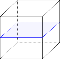
A hyperplane in is the union of all midcubes meeting the equivalence class of an edge (under the equivalence relation generated by square equivalence). A few facts about hyperplanes:
- A hyperplane meets each cube in at most one midcube.
- A hyperplane separates into two components.
- The cube structure on induces a cube structure on any hyperplane in .
1.5. Tangent: ends of groups
Let be any finitely generated group, with  being the set of generators. Then the number of ends of , denoted
  , is the number of components of the boundary
  . It’s a classic fact that the number of ends can only equal 0 (when is finite), 1 (e.g.
  ), 2 (e.g.
  ), or infinity (e.g. ).
The number of ends of a finitely generated group relative to a subgroup , denoted  , is the number of ends of the graph
  , i.e. the quotient of the Cayley graph of by the action of . Equivalently, it is the number of ends of the graph in which vertices are cosets of and vertices
  and
and  are connected if and only if
  .
.
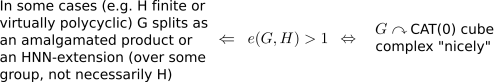
It is a famous result of Stallings that  if and only if splits as an amalgamated product or an HNN-extension over a finite group. In the language of Bass-Serre theory, we have:

For relative ends, the picture is more complicated:
The one of the key theorems which embody the ( ) implication above is the Algebraic Torus Theorem (Dunwoody-Swenson), given below. First, however, we must establish the subgroup with respect to which has multiple ends.
Theorem 3 (Sageev). Suppose  , a finite dimensional cube complex, without a global fixed point. Then there is a hyperplane
  such that
  .
.
Theorem 4 (Algebraic Torus). Suppose is finitely generated, and , a subgroup of , is virtually polycyclic with  . Then one of the following holds.
- is virtually polycyclic.
- There exists a short exact sequence

in which  is virtually polycyclic and
  is non-elementary fuchsian (see below).
- splits over a virtually polycyclic group.
1.6. Tangent: fuchsian groups
A fuchsian group is a subgroup of  . Thus, a fuchsian group acts discretely on the hyperbolic plane
  . Consider the set
  , for some
  . With respect to the hyperbolic metric on , the set has no limit points: either in , since the action is discrete, or in
  , since every point in is infinitely far from the boundary. However, considering the Euclidean distance inherits by being embedded as the Poincaré disk in
  , may have limit points in . Basic hyperbolic geometry implies that:
- the limit points occur only in ,
- for any other
 , the sets of limit points of
  and are identical, and
- the cardinality of the set of limit points is 0, 1, 2 or uncountable.
A fuchsian group is non-elementary when the set of limit points is uncountable. Such a group contains .
The non-elementary fuchsian groups are really the only interesting ones: the elementary ones are either finite or virtually cyclic.
Let’s recap the proof so far. We proceed by induction, and assume the theorem true for  . For of dimension , since is infinite and acts properly on , it has no global fixed points. Hence we apply Sageev’s theorem and conclude that there is a hyperplane s.t. . Let
  . Then acts on
  properly. By induction, either has an subgroup, and then so does so we’re done, or is virtually f.g. abelian. In this case, we apply the Algebraic Torus Theorem to and , and conclude that (1) is virtually polycyclic, or (2) it has a non-elementary fuchsian quotient, or (3) it splits over a virtually polycyclic group. We deal with these possibilities one by one.
If is virtually polycyclic, then we can apply the following two results of Bridson to conclude that it’s in fact virtually abelian.
Lemma 5.
- If , a complex with finitely many shapes, then acts semi-simply with a discrete set of translation lengths.
- If acts semi-simply and properly on a space, then any virtually solvable subgroup is virtually abelian.
(The number of shapes of a metric cell complex is the number distinct isometry classes of cells. In our case, has finitely many shapes since every cube of a given dimension is isometric and is has finite dimension. An action is semi-simple if there are points in the space realizing the translation lengths of each element. I.e., if for every  there’s a point realizing
  ).
).
If has a non-elementary fuchsian quotient, which must contain an , then itself must contain an .
Finally, suppose splits over a virtually polycyclic group . Then by the first part of Bridson’s lemma above, acts semi-simply, and by the second part, must be virtually abelian. We analyze amalgamated products and HNN-extensions separately.
Suppose  . If
. If ![{[A:P] > 2}](https://s0.wp.com/latex.php?latex=%7B%5BA%3AP%5D+%3E+2%7D&bg=ffffff&fg=000000&s=0&c=20201002) or
or ![{[B:P]>2}](https://s0.wp.com/latex.php?latex=%7B%5BB%3AP%5D%3E2%7D&bg=ffffff&fg=000000&s=0&c=20201002) , then contains an , by the normal form theorem for amalgamated products. If
, then contains an , by the normal form theorem for amalgamated products. If ![{[A:P] = [B:P] = 2}](https://s0.wp.com/latex.php?latex=%7B%5BA%3AP%5D+%3D+%5BB%3AP%5D+%3D+2%7D&bg=ffffff&fg=000000&s=0&c=20201002) , then the Bass-Serre tree, on which acts, is homeomorphic to a line in which every edge is stabilized by a conjugate of . Thus there’s an index 2 subgroup
, then the Bass-Serre tree, on which acts, is homeomorphic to a line in which every edge is stabilized by a conjugate of . Thus there’s an index 2 subgroup  acting by translations and
  . Hence
  , and so is virtually polycyclic and hence virtually abelian by Bridson’s lemma. This takes care of the amalgamated product case. To analyze an HNN-extension by , as well as to prove this theorem for non-finitely generated , another theorem is required.
Theorem 6 (Bridson-Haefliger). Suppose by semi-simple isometries and is . Suppose also that
- there’s a bound on the dimension of isometrically embedded flats,
- the set of translation lengths of is discrete at 0, and
- there is a bound on the order of finite subgroups.
Then any ascending sequence of virtually abelian subgroups stabilizes.
Suppose  , with
  and
and  being the two injections of into
  . If
. If ![{[C:i_1(P)] > 1}](https://s0.wp.com/latex.php?latex=%7B%5BC%3Ai_1%28P%29%5D+%3E+1%7D&bg=ffffff&fg=000000&s=0&c=20201002) and
and ![{[C:i_2(P)] > 1}](https://s0.wp.com/latex.php?latex=%7B%5BC%3Ai_2%28P%29%5D+%3E+1%7D&bg=ffffff&fg=000000&s=0&c=20201002) , then by the normal form theorem for HNN-extensions, has an subgroup. If
, then by the normal form theorem for HNN-extensions, has an subgroup. If ![{[C:i_1(P)] = 1}](https://s0.wp.com/latex.php?latex=%7B%5BC%3Ai_1%28P%29%5D+%3D+1%7D&bg=ffffff&fg=000000&s=0&c=20201002) , then
, then ![{[C:i_2(P)] = 1}](https://s0.wp.com/latex.php?latex=%7B%5BC%3Ai_2%28P%29%5D+%3D+1%7D&bg=ffffff&fg=000000&s=0&c=20201002) . [Otherwise, if
. [Otherwise, if  , consider the following subgroups of :

By the Bridson-Haefliger theorem above, this sequence must stabilize, hence  .] Then
  , and by Bridson’s lemma, is virtually abelian.
This finishes the proof for finitely generated . If is not finitely generated, it contains an ascending, non-stabilizing sequence of finitely generated subgroups
If any  contains an , we’re done. If not, then by the theorem applied to finitely generated groups, each is virtually abelian. Then conditions of the Bridson-Haefliger theorem above are satisfied, however, so a non-stabilizing ascending sequence is impossible. Hence if is not finitely generated, it contains an .

 to a continuous
  is called a Cannon-Thurston map. By the continuity of
  , if such a map exists it’s unique.
 , where
  is a hyperbolic closed 3-manifold fibering over a circle, and
  , where
  is an infinite hyperbolic normal subgroup of a hyperbolic group
  . Then there exists a Cannon-Thurston map
  be a finite graph of groups where all vertex groups
  and edge groups
  are hyperbolic, and all injections
  (where
  is incident to
  ) are quasi-isometric embeddings. Suppose that
  is also hyperbolic. Then for any vertex
  , there is a Cannon-Thurston map
  .
.
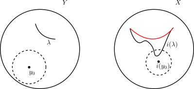
 be a proper embedding of proper hyperbolic spaces. Suppose, given
  , that there is a non-negative function
  such that
  as
as  and for all geodesic segments
  outside an
  -ball around
  is outside the
  (see the illustration below). Then there’s a Cannon-Thurston map
  .
. 
 does not extend continuously, there exist sequences
  in
in  such that
  and
and  for some
  , but
, but  and
and  for
for  in
in  .
.![{d_Y(y_0, [x_m,y_m]) \rightarrow \infty}](https://s0.wp.com/latex.php?latex=%7Bd_Y%28y_0%2C+%5Bx_m%2Cy_m%5D%29+%5Crightarrow+%5Cinfty%7D&bg=ffffff&fg=000000&s=0&c=20201002) as
as  . On the other hand, for
  large enough,
 ![{d_X(i(y_0), [i(x_m),i(y_m)])}](https://s0.wp.com/latex.php?latex=%7Bd_X%28i%28y_0%29%2C+%5Bi%28x_m%29%2Ci%28y_m%29%5D%29%7D&bg=ffffff&fg=000000&s=0&c=20201002) stays uniformly close to
stays uniformly close to ![{d_X(i(y_0),[u,v]) > 0}](https://s0.wp.com/latex.php?latex=%7Bd_X%28i%28y_0%29%2C%5Bu%2Cv%5D%29+%3E+0%7D&bg=ffffff&fg=000000&s=0&c=20201002) (see the discussion of visibility in the
(see the discussion of visibility in the 
 of hyperbolic metric spaces is a metric space
  admitting a map
  onto a simplicial tree
  satisfying
  ,
,  is path connected, rectifiable, and
  -hyperbolic. We denote the induced path metric by
  .
.
 are uniformly proper. That is, there exists a function
  such that for all
  , if
, if  , then
  .
.
 ,
,  is path connected and rectifiable. The induced path metric is denoted
  .
.
![{f_e: X_e \times [0,1] \rightarrow X}](https://s0.wp.com/latex.php?latex=%7Bf_e%3A+X_e+%5Ctimes+%5B0%2C1%5D+%5Crightarrow+X%7D&bg=ffffff&fg=000000&s=0&c=20201002) such that
such that  is an isometry onto
  .
.
 and
and  are
are  -quasi-isometric embeddings into
  and
and  , where
  and
and  .
.
 such that for any
  , then
  , and
, and  as
as  .
. . In order to shortcut an
  -geodesic from
  to
to  , we can’t use a path that travels to more than
  other vertex spaces
  , since the distance between such subspaces is at least 1. The length of a path in
  which goes to infinity like
  as
as  increases.]
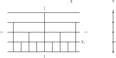
 is glued to the upper vertex subspace by an isometry and to the lower vertex subspace by a
  -quasi-isometry stretching the metric by a factor of 2.
 be a tree of hyperbolic metric spaces. If
  in
in  is constructed containing
  , then
  is outside an
  . Applying the key lemma above finishes the proof.
 intersecting
  is distance 1 away from
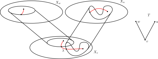
 when
when  with
with  , consider its universal cover
  (with the corresponding vertex and edge group assignments, so that
  ; see below for an example).
![\times [0,1]](https://s0.wp.com/latex.php?latex=%5Ctimes+%5B0%2C1%5D&bg=ffffff&fg=000000&s=0&c=20201002) and the corresponding quasi-isometric embeddings, we get a tree of hyperbolic spaces satisfying the hypotheses of Mitra’s theorem.
and the corresponding quasi-isometric embeddings, we get a tree of hyperbolic spaces satisfying the hypotheses of Mitra’s theorem. of hyperbolic groups to the boundaries
  . It is not evident that such maps should exist when
  . References include the textbooks of
 . Then
  is the set of equivalence classes of geodesic rays
  originating at
  (i.e.,
  ). Ray
  is equivalent to
  , written
  , if
, if  , or equivalently if the images of
  is the set of equivalence classes of quasigeodesic rays (originating at any point in the space). Here we must use only the finite Hausdorff distance as the equivalence relation. [Note: this definition has no analogue for CAT(0) spaces, where there is no quasigeodesic stability.]
 of generalized geodesic rays representing the points
  , i.e. geodesic segments connecting the basepoint
 ![{[0,\infty]}](https://s0.wp.com/latex.php?latex=%7B%5B0%2C%5Cinfty%5D%7D&bg=ffffff&fg=000000&s=0&c=20201002) by the constant map at
by the constant map at  So
So  A subsequence converges to a geodesic ray from
  . See the illustration below.)
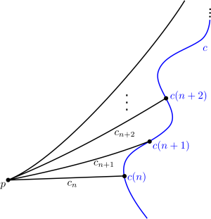
 as
as  for
for  if they are represented by generalized rays (geodesic rays allowed)
  from
from  has itself a subsequence converging to
 , a fundamental system of open sets in
  about
about  is the collection of
  , where a generalized ray
  if
if  . (The choice of
  does not matter since asymptotic rays from a fixed basepoint in a hyperbolic space are uniformly close: within
  of each other.)
 as
as  continuous).
 denote the set of continuous functions from
  with the
  , where
  if
if  is a constant map, by associating to
  the equivalence class of the distance to
  . The point of
  associated to a geodesic ray
  is represented by the Busemann function
  defined as
![\displaystyle b_c(x)=\limsup_{t\rightarrow\infty}{\left[d(x,c(t))-t\right]}.](https://s0.wp.com/latex.php?latex=%5Cdisplaystyle+b_c%28x%29%3D%5Climsup_%7Bt%5Crightarrow%5Cinfty%7D%7B%5Cleft%5Bd%28x%2Cc%28t%29%29-t%5Cright%5D%7D.&bg=ffffff&fg=000000&s=0&c=20201002)
 with the classical
  instead of near 0.
  are represented by sequences in
  :
:
![\displaystyle (x\cdot y)_z=\frac12\left[d(x,z)+d(y,z)-d(x,y)\right].](https://s0.wp.com/latex.php?latex=%5Cdisplaystyle+%28x%5Ccdot+y%29_z%3D%5Cfrac12%5Cleft%5Bd%28x%2Cz%29%2Bd%28y%2Cz%29-d%28x%2Cy%29%5Cright%5D.&bg=ffffff&fg=000000&s=0&c=20201002)
![{[z,x]}](https://s0.wp.com/latex.php?latex=%7B%5Bz%2Cx%5D%7D&bg=ffffff&fg=000000&s=0&c=20201002) and
and ![{[z,y]}](https://s0.wp.com/latex.php?latex=%7B%5Bz%2Cy%5D%7D&bg=ffffff&fg=000000&s=0&c=20201002) , or equivalently the distance from
, or equivalently the distance from  to
to ![{[x,y]}](https://s0.wp.com/latex.php?latex=%7B%5Bx%2Cy%5D%7D&bg=ffffff&fg=000000&s=0&c=20201002) . In a
. In a ![{d(z,[x,y])}](https://s0.wp.com/latex.php?latex=%7Bd%28z%2C%5Bx%2Cy%5D%29%7D&bg=ffffff&fg=000000&s=0&c=20201002) (to within some fixed multiple of
(to within some fixed multiple of  is said to converge at infinity if
  as
as  , and two such sequences
  converge to the same point if
  . (Transitivity of this relation follows from one of the many equivalent definitions of
  for all
  .) A fundamental system of neighborhoods of a boundary point is given by bounding the Gromov overlap from below by a sequence of numbers approaching infinity.
  ,
,  , there is a geodesic
  with
with  ,
,  . Indeed, take geodesic rays
  originating from a basepoint
  . Since
  (shown in blue) a distance more than
  . For
. For  , we can choose geodesic segments
  to
to  , and extend them to generalized geodesic lines. By
  , which we can assume is
  (shown in red). Then Arzelà–Ascoli gives a subsequence of
  is within
  for
for  and within
  of
of  . (See the diagram below.) So
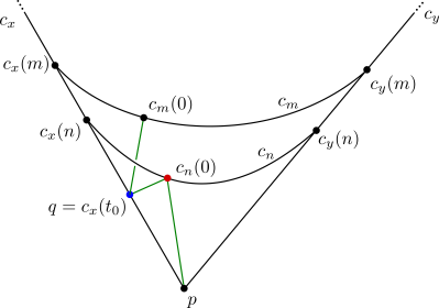
 between hyperbolic spaces, there is at most one way to extend it continuously to the boundary
  .
. is a (continuous) embedding, where
  (using the quasigeodesic model
  of hyperbolic boundary.) If
  is a quasi-isometry, then
  , so
, so  unless
  .
. to a hyperbolic group
  and
and  .
.  is a Cantor set.
![{M=(S\times[0,1])/((x,0)\sim(\phi(x),1))}](https://s0.wp.com/latex.php?latex=%7BM%3D%28S%5Ctimes%5B0%2C1%5D%29%2F%28%28x%2C0%29%5Csim%28%5Cphi%28x%29%2C1%29%29%7D&bg=ffffff&fg=000000&s=0&c=20201002) of a hyperbolic surface
of a hyperbolic surface  is a hyperbolic 3-manifold if and only if
  is an HNN-extension of a surface group
  , with
 , a space-filling curve. Therefore
  via its inclusion in
  : the set of accumulation points in
  of any
  Since
Since  of
of  . Therefore
  (The interior of a ball together with some points on its boundary is alway convex, after all.) So
  .
. . A projective resolution of a
  is an exact sequence
 is a projective
  as a trivial
  of a group
  such that
 have the property that their finitely presented subgroups are also hyperbolic. This result appears in Gersten’s paper
  is a group and
  is a finitely generated
  –module. Let
  be a finitely generated free
  , such that there is a surjective homomorphism
  of
of  is a free
  –basis for
  –norm
–norm  .
. . Such a norm
  on
on  and
and  is obtained from another surjective homomorphism from a different finitely generated free
  –module
  , then there is a uniform constant
  such that
  for all
  . So
. So 
 is free and finitely generated and given an
  associated to some basis, and
 is projective.
 for
for  (that is, a map
  is the identity on
  so that
  for all
  .
. is projective, we know that
  . We choose a map
  such that
  is the identity on
  be a finitely generated free submodule generated by a subset of the generators of
  which contains the image of
  . Let
. Let  . Notice that
  is also free, but not necessarily finitely generated. We can modify the retraction
  to
to  and
and  . Let
. Let  be a surjective homomorphism of
  such that
  . This map
  can be extended to
  by setting the images under
  . It follows this
  and
and  .
. are both finitely generated and free. So the map
  for all
  . Since the standard norm on
  for all
  . This completes the proof.
 be an arbitrary group and let
  . Then there exists an
  -dimensional
  -complex
  . If
. If  -complex.
 be a finitely presented group. So
  , where
  and
and  is the normal closure of the relations
  . Let the presentation
  –complex of this group be
  , the abelianization of R , and the
  –action on it is induced by the conjugation of
  –module structure on
  , where
  is the
  -skeleton of the universal cover of the presentation complex
  –complex
  .
. is an exact sequence of
  projective, then
  is projective.
 are projective and
  is projective.
 –modules
  . By definition this means that
  such that
  as
as  free as a
  of
of  and
and  satisfy
  . Further, by adding trivial letters and corresponding relations to the presentation for
  . An application of the
  is projective as a
 .
.  for
for  , such that there is a uniform constant
  with the property that
  for all
  . So if
  , then
  .
.  be a circuit in
  and let
  be a
be a  of minimal area. The area of
  , where
  is the element of
  corresponding to
  , where now
  is in terms of
  as a
as a  satisfies a linear isoperimetric inequality, then so does
  . Since
  . Hyperbolic groups are always of type
  is a branching locus if it satisfies the following two conditions:
 -cell
-cell  of
of  , we have that
  is a disjoint union of faces of
  .
. is nonempty and connected for each cell
  .
. , the link
  is a full subcomplex of
  .
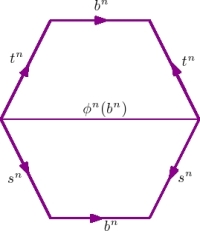
. is obtained as follows:
 .
.
 . If
. If  and let
  .
.
 , which is an example of a branching locus.
 :
: 
 is free of rank
  . As a free basis, take the six loops
  . (The bars indicate paths traversed in the opposite direction to their orientations.) Let
  be the homomorphism such that
 and
and  are the permutations
  and
and  , respectively. The essential feature of this construction is that
  maps all commutators of
  or
or  with
with  or
or  to non–trivial five–cycles, since
  .
.  , let
, let  be the projections
  ,
,  and
and  . All are continuous, onto, and induce homomorphisms
  .
.  be a retract
  to
to  . For
. For  .
.  defines a
  -fold covering of
  be the natural map
  .
. is hyperbolic
 space. By the following two theorems, to establish that
  –hyperbolic metric space. Then
  is a complete bipartite graph where each component has four vertices (along with some half edges i.e. edges with one end–point missing). Each loop is this graph that consists of four edges maps to the boundary of a neighborhood of a point in
  under exactly one of the maps
  or
or  . Such a loop deformation retracts to one of the commutator loops in
  . Therefore in the branched cover, the link structure around these vertices is distorted, i.e. the aforementioned loops lift to
  –fold copies.
 in the universal cover intersecting this plane that is not parallel to it, which maps to an edge in the branching locus. Let the intersection of the flat plane with this edge be
  . The link of
  give rise to a map to the oriented unit circle mapping the edges to the cirlce respecting the orientation. This extends linearly to a map
  .
. lifts to a map from the universal cover of
  . The ascending and descending links of any vertex in this Morse theory setting are
  induced by
  , and in particular not hyperbolic. For further details of such Combinatorial Morse theory, see
  but not of type
  be a presentation complex for some presentation of
  is a loop in
  , we define the filling area of

 , or equivalently if and only if
  is subquadratic. This result is due to Gromov; the absence of Dehn functions between linear and quadratic is called the “Gromov Gap”.
 . (On account of the Gromov gap, this means that
  or
or  .)
.)
 .
. such that
  is a short exact sequence,
  .
. and is defined by
  . The automorphism
  is given by
  and
and  . Let
. Let  , the free group generated by
  and
and  . You can see that
  by considering the family of words
  (with length on the order of

 letters, and it is clearly reduced in
  , where
  . The corresponding presentation complex built out of squares can be shown to satisfy the link condition.
 of
of  .
.  . Alternatively, see
  , for a proof see Theorem 6.20 in
  . Now consider the following family of embedded disks in
  :
:
 . Moreover, the boundary loops of these disks do not admit fillings with smaller area, since
  -dimensional and aspherical. (In such spaces the embedded filling is the most efficient among the fillings of any loop.) This shows that
  is a lower bound on the Dehn function.
  embeds in
  . Since
  . Then the subgroup
  of
of  . (It is easy to see that the relations
  and
and  , and the corresponding relations involving
  and
and  in Step 1, one can construct other examples.
 , where
  is a CAT(0) group, and
  . (The example above is the case n=2.) Then the double
  embeds in
  , and
, and  . Thus,
  occurs as the Dehn function of a subgroup of a CAT(0) group for all integers
  .
.  be a hyperbolic surface bundle over a circle. Then one has a short exact sequence
  , and
, and  is a CAT(0) group. Bridson and Haefliger prove that if
  . Hence,
  and
and  . In fact it is
  . Thus,
  occurs as the Dehn function of a subgroup of a CAT(0) groups.
 to use in Step 1, for example due to
  for
for  or functions growing faster than
  .
.
 . The lower bound was proved in a manner similar to the example above, by constructing a sequence of embedded diagrams in the level set for
  .
.
 , where
  is not an integer, but
  has Dehn function
  .
.  . Using these in Step 1 of the Bieri doubling trick, they produce a class of examples of subgroups of CAT(0) groups with Dehn functions of the form
  is an integer. The kernels are of type
  , unlike the original Bieri doubles, which all have finite
  ‘s. Another interesting direction is to study higher dimensional Dehn functions of CAT(0) groups and their subgroups. We won’t go into the technicalities here, but just say that the
  measures the difficulty of filling
  -chains (or
  . (As in the case
  , the group
  attains this general upper bound.)
 such that there is no algorithm to decide membership of
  has a solvable conjugacy problem (
 where
where 
 is finitely presented and
  , and so questions about equality in
 ),
), 
 , can be identified with to a finite presentation
  of
of  is finitely generated as a
  is finite. This can be seen by taking the attaching maps of the 3-cells as the generators of the module. This identification allows one to find a nice presentation for
  be a presentation for a group
  be a sequence of words of the form
  where
where  and
and  is some word over
  . We call such a sequence an identity sequence if
  is freely equal to the empty word in
  . An equivalence relation is given on identity sequences, and we consider the action of
  . This action naturally induces a
  . Thus
  , a compact, negatively curved, piecewise hyperbolic 2-dimensional complex
 ,
,
 ,
,
 of cardinality at least 2,
 is represented by one of the 1-cells of
  follows from the next result.
 such that
  and unsolvable word problem. The enhanced Rips construction is applied to to
  , where
  where
where  and the
  are lifts of generators of
  for a generating set for
  is in
is in  be finitely generated groups. Suppose
  and there exists
  such that
  . If there is no algorithm to decide membership of
  where
where  , as item (9) of Theorem 3 tells us that the centralizer of
  is
is  , and thereby gives us unsolvability of the conjugacy problem.
 and
and 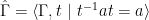 is the fundamental group of a compact non=-positively curved squared complex, and is thus biautomatic (
 such that there is no algorithm to determine whether or not
  is isomorphic to
  .
.  where
where  is an HNN-extension of
  where
where  generates a maximal cyclic subgroup.
 ,
,  ,…. Hercules fights a hydra by striking off its first letter. The hydra then regenerates as follows: each remaining letter
  , where
  , becomes
  and the
  .
. 
 in five strikes:
 to be the number of strikes it takes Hercules to vanquish the hydra
  ,
,  , define
  . For example,
  and
and  (another fun exercise).
  , defined for integers
  by:
by:  and
and  . So, in particular,
  ,
,  and
and  , the
, the  is essentially a version of Ackermann’s function:
  .
. is a hydra (
 ). Then in the time
  it takes to kill
  (and many other letters besides) after the final
  . Disposing of those letters then represents an additional challenge for Hercules. So the time it takes to complete that initial task of killing

 ,
,
 is a rank–
 .
.![{[a_1,t]=1}](https://s0.wp.com/latex.php?latex=%7B%5Ba_1%2Ct%5D%3D1%7D&bg=ffffff&fg=000000&s=0&c=20201002) and
and ![{a_{i-1} = [a_i,t]}](https://s0.wp.com/latex.php?latex=%7Ba_%7Bi-1%7D+%3D+%5Ba_i%2Ct%5D%7D&bg=ffffff&fg=000000&s=0&c=20201002) for
for  (convention:
 ![{[a,b]= a^{-1}b^{-1}ab}](https://s0.wp.com/latex.php?latex=%7B%5Ba%2Cb%5D%3D+a%5E%7B-1%7Db%5E%7B-1%7Dab%7D&bg=ffffff&fg=000000&s=0&c=20201002) ) and then eliminating
) and then eliminating  and defining
  , one can present
 ![\displaystyle G_k \ \cong \ \langle \ a, t \ \mid \ [a, \underbrace{t, \ldots, t}_k ] =1 \ \rangle.](https://s0.wp.com/latex.php?latex=%5Cdisplaystyle+G_k+%5C+%5Ccong+%5C+%5Clangle+%5C+a%2C+t+%5C+%5Cmid+%5C+%5Ba%2C+%5Cunderbrace%7Bt%2C+%5Cldots%2C+t%7D_k+%5D+%3D1+%5C+%5Crangle.&bg=ffffff&fg=000000&s=0&c=20201002)
 where
where  is the “Engel” word defined recursively by
  and
and ![{v_{i+1} = [v_i,t]}](https://s0.wp.com/latex.php?latex=%7Bv_%7Bi%2B1%7D+%3D+%5Bv_i%2Ct%5D%7D&bg=ffffff&fg=000000&s=0&c=20201002) for
for  .
. and
and 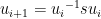 for
for  for every
  in
in  , the words
  and
and  become freely equal for all
  . So the relation
  to give an alternative one–relator presentation for
 for
for  as
as 
 that represents the identity. So when the
  ‘s are carried through the word and collected at the end (using the defining relations of
  is
is  ?
?
 and
and  . One can try to convert
  to a word on
  and
and  times a power of
  to pair the first letter with
  to the end of the word by conjugating through the intervening letters; then pair off the next

 .
.

 denote the reduced word on
  which represents
  . The diagram pictured above can be paired with its mirror image, separated by three corridors of 2–cells as shown below, to give a diagram that demonstrates the equality in
  (the word along the bottom of the diagram) to a word of length
  . Thus the distortion is at least
  .
. 
![{\langle G_k, p \mid [p, a_it]=1 \ (\forall i) \rangle}](https://s0.wp.com/latex.php?latex=%7B%5Clangle+G_k%2C+p+%5Cmid+%5Bp%2C+a_it%5D%3D1+%5C+%28%5Cforall+i%29++%5Crangle%7D&bg=ffffff&fg=000000&s=0&c=20201002)
 .
. with a free rank–
 subgroup
  whose distortion is
  .
. 

 are some words on the
  which we won’t specify explicitly here. So comparing with
  and the seventeen
  that is present in
  is an automorphism.
 but the
  . [The number of
  is
is  and
and  do not depend on
 and
and  . All the other defining relations are encoded in the graphs: an edge labelled
  . I won’t explain here why these presentations both give
  –valued Morse function all of whose ascending and descending links are trees, then its fundamental group is free–by–cyclic. (See, for example,
  , the four green edges have length
  , and all other edges have length
  .]
.]
 , and then checking that no cells have all their corners giving rise to edges in the list.
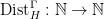 of a finitely generated subgroup
 and
and  denote word metrics associated to some choices of finite generating sets. Those choices are not important: different choices lead to
  –equivalent distortion functions.
  (in the sense of
  and this leads to the Dehn functions being at least as fast growing as the distortion functions: if a short word
  in this
  , then
 ![{[a,w]}](https://s0.wp.com/latex.php?latex=%7B%5Ba%2Cw%5D%7D&bg=ffffff&fg=000000&s=0&c=20201002) represents the identity and has area at least
represents the identity and has area at least 

 when it conjugates
  , graphically displays this calculation.
 . Then the distortion of
 . [We will write
  for the

 . [We will not go into details of the upper bounds, it suffices to say they do not harbour any great subtleties.] Here is an illustration of the calculation that leads to the 3–fold iterated exponential distortion:

 , we can re–express this presentation as:
 and so the distortion grows like
  .
. 

 and
and  . This is an exponentially growing automorphism — that is,
  has length
  when re–expressed as a minimal length word in

 is a Euclidean square and those corresponding to
  and
and  are Euclidean equilateral triangles, all of side–length
 takes
takes  to a conjugate of itself or its inverse. It follows that
  has a
has a  –subgroup and so is not hyperbolic.] The existence of hyperbolic free–by–cyclic and, more generally, free–by–free examples can be derived from
  or, faster, like
  . These examples combine the techniques we’ve seen above for free–by–cyclic and the iterated Baumslag–Solitar groups. The idea of uniting these ideas to give hyperbolic examples is due to
 and the
  are positive words on
  of length
  with the property that each two letter–word
  appears at most once as a subword of the
 , and in which no
  appears twice as a subword. In the same manner as the free–by–cyclic example described earlier they get:
 is free of rank–
 .
. 
 and
and  is always at least
  . Accordingly, Barnard–Brady–Dani describe the free subgroup generated by the
  as highly convex — this will be important momentarily.
 is a free group of rank
  which is identified with the exponentially distorted subgroup in
  and the highly convex subgroup in
  . So we have exponential–upon–exponential–upon–exponential… distortion leading to
  being distorted
  . One can build a presentation 2–complex for a presentation of
  ,
,  , …,
, …,  , define
 positive words of length
  are
are  subword occurring twice among any of them. Again, find these
  and
and  will work).
  .
. 