Boundaries of Hyperbolic Groups

In this post and the next, we will discuss Cannon-Thurston maps: (continuous) extensions of inclusions ${H\leq G}$ of hyperbolic groups to the boundaries ${\partial H\rightarrow\partial G}$ . It is not evident that such maps should exist when ${H}$ is distorted in ${G}$ , but they often do nonetheless. This post will focus on defining the boundary of a hyperbolic group and establishing basic properties. We’ll take a brief look at Cannon-Thurston‘s first (distorted) example. The next post will discuss the progress of Mitra towards the following open question:

Question: If ${H\leq G}$ are hyperbolic groups, does there exist a Cannon-Thurston map ${\partial H\rightarrow\partial G}$ ?

In particular, he has answered the question in the affirmative for the case of normal hyperbolic subgroups of hyperbolic groups and vertex subgroups of finite hyperbolic graphs of hyperbolic groups with quasi-isometric edge inclusion maps.

1. The boundary of a Gromov-hyperbolic space

In this section, ${X}$ is a geodesic space that is proper and hyperbolic. We’ll see several equivalent definitions for ${\partial X}$ and the closure ${\overline{X}:=X\cup\partial X}$ . References include the textbooks of Bridson-Haefliger and Ghys-de la Harpe (in French) and Kapovich-Benakli’s survey paper Boundaries of Hyperbolic Groups.

Here are two examples to keep in mind. Morally, the boundary of the hyperbolic plane should be the circle at infinity in the Poincare disk model. The boundary of the Cayley graph ${\Gamma}$ for ${F_2}$ should be a Cantor set, which can be viewed (under the “obvious” embedding of the Cantor set in the plane – see picture below) as the set of limit points of ${\Gamma}$ not in ${\Gamma}$ itself. Note: the Cantor set is totally disconnected, so the set of ends is the same as the boundary.

Geodesic rays will be parametrized by arclength.

Fix a basepoint ${p\in X}$ . Then ${\partial(X,p)}$ is the set of equivalence classes of geodesic rays ${c:[0,\infty)\rightarrow X}$ originating at ${p}$ (i.e., ${c(0)=p}$ ). Ray ${c_1}$ is equivalent to ${c_2}$ , written ${c_1(\infty)=c_2(\infty)}$ , if ${\sup_t{d(c_1(t),c_2(t))}<\infty}$ , or equivalently if the images of ${c_1}$ and ${c_2}$ are a finite Hausdorff distance from each other. [Note: for CAT(0) spaces, each equivalence class contains a single ray since the metric is convex.]
${\partial X}$ is defined the same way, but without requiring that rays originate at ${p}$ .
${\partial_qX}$ is the set of equivalence classes of quasigeodesic rays (originating at any point in the space). Here we must use only the finite Hausdorff distance as the equivalence relation. [Note: this definition has no analogue for CAT(0) spaces, where there is no quasigeodesic stability.]

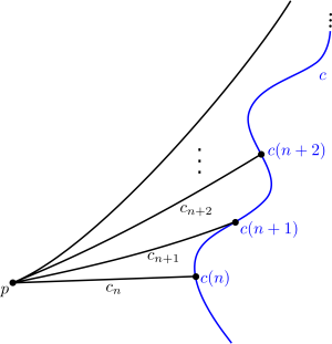
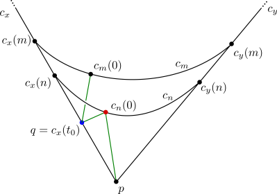
These three sets are in natural bijection: As equivalence classes in (1) are contained in equivalence classes in (2) which are contained in equivalence classes in (3), we need only check that each quasigeodesic equivalence class contains a geodesic ray starting at ${p}$ . This follows from the Arzelà–Ascoli theorem and quasigeodesic stability. (Take a sequence ${c_n}$ of generalized geodesic rays representing the points ${c(n)}$ , i.e. geodesic segments connecting the basepoint ${p}$ to ${c(n)}$ with domain extended to ${[0,\infty]}$ by the constant map at ${c(n).}$ So ${c_n(\infty)=c(n).}$ A subsequence converges to a geodesic ray from ${p}$ which is Hausdorff-close to ${c}$ . See the illustration below.)

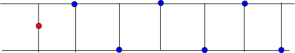
To topologize these boundaries, it suffices to topologize ${\partial(X,p)}$ . We do this by defining convergence: ${x_n\rightarrow x}$ as ${n\rightarrow\infty}$ for ${x_n,x\in\overline{(X,p)}}$ if they are represented by generalized rays (geodesic rays allowed) ${c_n,c}$ from ${p}$ such that every subsequence of ${\{c_n\}}$ has itself a subsequence converging to ${c}$ pointwise and uniformly on compact sets. It is necessary to take subsequences here because we want the sequence of blue points below with red basepoint to converge (to a single point on the boundary):

Closed sets are defined to be the sets containing all their limit points. For any fixed ${k>2\delta}$ , a fundamental system of open sets in ${\overline{X}}$ about ${c\in\partial(X,p)}$ is the collection of ${V_n(c)}$ , where a generalized ray ${c'\in V_n(c)}$ if ${d(c(n),c'(n))<k}$ . (The choice of ${k}$ does not matter since asymptotic rays from a fixed basepoint in a hyperbolic space are uniformly close: within ${2\delta}$ of each other.)

This difficulty requiring us to take subsequences does not arise in defining the boundary of CAT(0) spaces, since the metric is convex. If ${X}$ is both hyperbolic and CAT(0), the various ${\overline{X}}$ defined above are homeomorphic to the inverse limit of the closed balls ${\overline{B}(p,n)}$ as ${n}$ varies, induced by the projection maps to these complete convex subsets. The topology is the inverse limit topology (the coarsest topology making all the maps ${\overline{X}\rightarrow\overline{B}(p,n)}$ continuous).
Let ${\mathcal{C}(X,\mathbb{R})}$ denote the set of continuous functions from ${X}$ to ${\mathbb{R}}$ with the compact-open topology. Identify ${X}$ with a subset of ${\mathcal{C}(X,\mathbb{R})/\sim}$ , where ${f\sim g}$ if ${f-g}$ is a constant map, by associating to ${x\in X}$ the equivalence class of the distance to ${x}$ function: ${d(x,\cdot)}$ . The point of ${\partial X:=\overline{X}\setminus X}$ associated to a geodesic ray $c$ is represented by the Busemann function ${b_c}$ defined as
$\displaystyle b_c(x)=\limsup_{t\rightarrow\infty}{\left[d(x,c(t))-t\right]}.$

The level sets of Busemann fuctions are called horospheres, agreeing in ${\mathbb{H}^n}$ with the classical horospheres. A Busemann function can be viewed as a sort of “distance” function to a point of ${\partial X}$ , but with close points having very small distance: near ${-\infty}$ instead of near 0.
Points of the sequential boundary ${\partial_sX}$ are represented by sequences in ${X}$ that converge to a point in ${\partial X}$ . To describe this convergence, we’ll need to use the Gromov product for points ${x,y,z\in X}$ :
$\displaystyle (x\cdot y)_z=\frac12\left[d(x,z)+d(y,z)-d(x,y)\right].$

In a tree, the Gromov product represents the overlap length of the segments ${[z,x]}$ and ${[z,y]}$ , or equivalently the distance from ${z}$ to ${[x,y]}$ . In a ${\delta}$ -hyperbolic space, the Gromov product gives a good proxy for ${d(z,[x,y])}$ (to within some fixed multiple of ${\delta}$ , depending on the definition of ${\delta}$ -hyperbolicity used.)

Fix a basepoint ${p\in X}$ . A sequence ${x_n}$ is said to converge at infinity if ${(x_n\cdot x_m)_p\rightarrow\infty}$ as ${n,m\rightarrow\infty}$ , and two such sequences ${x_n,y_n}$ converge to the same point if ${(x_n\cdot y_m)_p\rightarrow\infty}$ . (Transitivity of this relation follows from one of the many equivalent definitions of ${\delta}$ -hyperbolicity: ${(x\cdot y)_w\geq\min((x\cdot z)_w,(y\cdot z)_w)-\delta}$ for all ${w,x,y,z\in X}$ .) A fundamental system of neighborhoods of a boundary point is given by bounding the Gromov overlap from below by a sequence of numbers approaching infinity.

2. Basic Properties

Most of these facts are taken from Bridson-Haefliger, chapter III.H.3.

Fact: ${\overline{X}}$ is compact. Arzelà–Ascoli gives sequential compactness, and compactness then follows from first countability.

Fact: ${\partial X}$ is visible: for every ${x,y\in\partial X}$ , ${x\neq y}$ , there is a geodesic ${c:\mathbb{R}\rightarrow X}$ with ${c(\infty)=x}$ , ${c(-\infty)=y}$ . Indeed, take geodesic rays ${c_x,c_y}$ originating from a basepoint ${p}$ with ${c_x(\infty)=x,c_y(\infty)=y}$ . Since ${x\neq y}$ , there is a point ${q=c_x(t_0)}$ (shown in blue) a distance more than ${\delta}$ away from ${c_y}$ . For ${n>t_0}$ , we can choose geodesic segments ${c_n}$ joining ${c_y(n)}$ to ${c_x(n)}$ , and extend them to generalized geodesic lines. By ${\delta}$ -hyperbolicity, some point of the segment ${c_n}$ is a distance less than ${\delta}$ from ${q}$ , which we can assume is ${c_n(0)}$ (shown in red). Then Arzelà–Ascoli gives a subsequence of ${c_n}$ converging to a bi-infinite geodesic ${c}$ . By ${\delta}$ -hyperbolicity, ${c_n(t)}$ is within ${2\delta}$ of ${c_x}$ for ${t>0}$ and within ${3\delta+d(p,q)}$ of ${c_y}$ for ${t<0}$ . (See the diagram below.) So ${c(\infty)=x}$ and ${c(-\infty)=y}$ .

Given a map ${f:X\rightarrow X'}$ between hyperbolic spaces, there is at most one way to extend it continuously to the boundary ${f_\partial:\partial X\rightarrow\partial X'}$ .

Fact: If ${f:X\rightarrow X'}$ is a quasi-isometric embedding of geodesic, proper, hyperbolic spaces then ${f_\partial}$ is a (continuous) embedding, where ${f_\partial(c)=f\circ c}$ (using the quasigeodesic model ${\partial_qX'}$ of hyperbolic boundary.) If ${f}$ is a quasi-isometry, then ${f_\partial}$ is a homeomorphism. (These statements follow immediately from quasigeodesic stability and the description of a fundamental base of neighborhoods ${V_n(c)}$ above.)

Example: ${\partial\mathbb{H}^n=S^{n-1}}$ , so ${\mathbb{H}^n}$ is not quasi-isometric to ${\mathbb{H}^m}$ unless ${n=m}$ .

Since the hyperbolic boundary is a quasi-isometry invariant, we can associate a boundary ${\partial G}$ to a hyperbolic group ${G}$ .

Example: If ${S}$ is a closed hyperbolic surface and ${M}$ a closed hyperbolic 3-manifold, then ${\partial\pi_1(S)=\partial\mathbb{H}^2=S^1}$ and ${\partial\pi_1(M)=\partial\mathbb{H}^3=S^2}$ .

Example: ${\partial F_2}$ is a Cantor set.

By the above fact, the inclusion map from an undistorted hyperbolic subgroup ${H}$ of a hyperbolic group ${G}$ extends to a continuous map (in fact, an embedding) ${\partial H\rightarrow\partial G}$ . When ${H}$ is an arbitrary hyperbolic subgroup of a hyperbolic group ${G}$ , a continuous (not necessarily injective) extension of the inclusion to ${\partial H\rightarrow\partial G}$ is called a Cannon-Thurston map.

3. Cannon and Thurston’s Example

Thurston proved that the mapping torus ${M=(S\times[0,1])/((x,0)\sim(\phi(x),1))}$ of a hyperbolic surface ${S}$ by a surface automorphism ${\phi}$ is a hyperbolic 3-manifold if and only if ${\phi}$ is pseudo-Anosov. In particular, there exist hyperbolic 3-manifolds where ${\pi_1M}$ is an HNN-extension of a surface group ${\pi_1S}$ , with

$\displaystyle 1\rightarrow\pi_1S\rightarrow\pi_1M\rightarrow\mathbb{Z}\rightarrow1.$

Cannon-Thurston showed the inclusion extends to a surjective map ${S^1=\partial H^2=\partial\pi_1S\rightarrow\partial\pi_1M=\partial\mathbb{H}^3=S^2}$ , a space-filling curve. Therefore ${\pi_1S}$ is a distorted subgroup of ${\pi_1M}$ . This was the first example found of a Cannon-Thurston map involving a distorted subgroup. (Mitra’s work, described in the next post, generalizes this result: he shows that there is a Cannon-Thurston map for any hyperbolic normal subgroup of a hyperbolic group.) We will sketch here why the map is surjective.

${\pi_1S}$ acts properly by isometries on ${\mathbb{H}^3}$ via its inclusion in ${\pi_1M}$ . The image of the Cannon-Thurston map is the limit set ${\Lambda\pi_1S}$ : the set of accumulation points in ${\partial\mathbb{H}^3}$ of any ${\pi_1S}$ -orbit in ${\mathbb{H}^3.}$ Since ${\pi_1S}$ is a normal subgroup, elements of ${\pi_1M}$ act on ${\mathbb{H}^3}$ by permuting these orbits, so they fix ${\Lambda\pi_1S}$ . Consequently, they fix the convex hull ${K}$ of ${\Lambda\pi_1S}$ in ${\overline{\mathbb{H}^3}}$ . Therefore ${K}$ contains a ${\pi_1S}$ -orbit which is quasi-isometric to ${\mathbb{H}^3}$ itself, so the closed set ${K}$ contains the whole boundary ${\partial\mathbb{H}^3}$ . But ${K\cap\partial\mathbb{H}^3=\Lambda\pi_1S.}$ (The interior of a ball together with some points on its boundary is alway convex, after all.) So ${\Lambda\pi_1S=\partial\mathbb{H}^3}$ .